← All modules

Chapter 3 · Transport in the Capillary–Tissue System

Solute transport in the retina

We use a prescribed retinal blood flow to study how solutes move through the capillary bed and exchange with surrounding tissue.

The vascular network

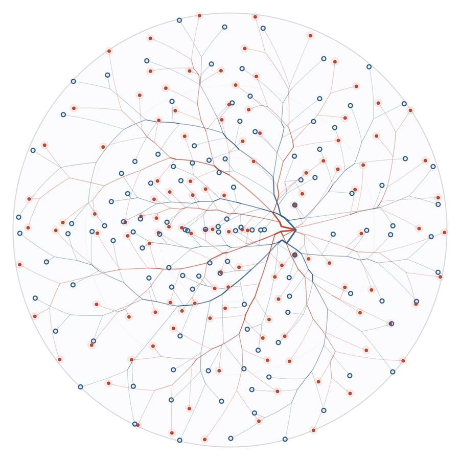
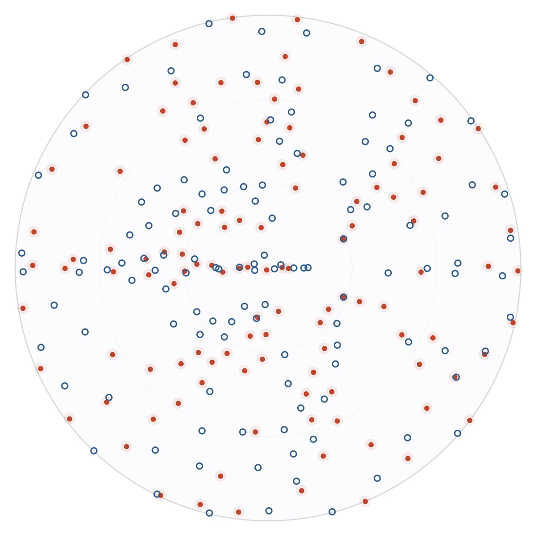
The surface vascular network and its 240 terminal positions on the same projected disk. The prescribed flow sets one signed volume flow at every terminal; the arterial tree supplies the capillary bed and the venous tree drains it.
Arterial and venous surface trees on the stereographic disk
Surface vascular network
Arterial and venous terminals on the projected disk
Arterial and venous terminals
Arterial terminal · given c = 1 Venous terminal · unknown Surface segment

Simplified caseThe simplified model uses prescribed terminal flows and sets arterial terminal concentrations to 1. The capillary bed supplies the concentration at each venous inlet.

The coupled system

Two concentration fields on the same spherical cap, coupled across the capillary wall and closed by terminal regions and flow-weighted mixing.

Vessels
1D advection along each segment; the arterial inlet carries concentration 1.
Capillary bed
Advection–diffusion with arterial injection, venous collection, and wall exchange.
Tissue
Advection–diffusion with wall exchange and a consumption sink.
Connections
Terminal averages, flow-weighted junction mixing, and zero normal flux at the rim.
2coupled media
240terminal vessels
476surface segments
1conservative balance

Governing equations

Let IA\mathcal I_A and IV\mathcal I_V denote the arterial and venous terminal sets. The prescribed terminal volume flow qnq_n is positive at an artery and negative at a vein, with ∑nqn=0\sum_n q_n=0. The prescribed arterial terminal concentration cA,nc_{A,n} is constant and set to 1 in the simplified case. The venous inlet concentration cV,n(t)c_{V,n}(t) is determined by solute collection from the capillary bed at time tt.

Transport evolves in time under fixed terminal flows and pressures from the Pressure Model. Use ⋆∈{cap,t}\star\in\{\mathrm{cap},\mathrm t\} to index the capillary bed and tissue.

Transport parameters
SymbolMeaning
HHEffective thickness
ε⋆\varepsilon_\starLiquid volume fraction
σ⋆=Hε⋆\sigma_\star=H\varepsilon_\starStorage coefficient
D⋆D_\starSpatially constant solute diffusivity
κ⋆\kappa_\starDarcy coefficient
αrΔπ\alpha_r\Delta\piOsmotic pressure correction, given by the reflection coefficient times the osmotic pressure difference
αsol\alpha_{\mathrm{sol}}Solute exchange coefficient
β\betaFirst-order tissue consumption rate

Spherical cap S\mathcal S

For medium ⋆∈{cap,t}\star\in\{\mathrm{cap},\mathrm t\} (capillary bed or tissue), p⋆,Sp_{\star,\mathcal S} is pressure and c⋆,Sc_{\star,\mathcal S} is normalized solute concentration. The subscripts on the differential operators denote the surface gradient, divergence, and Laplacian. The unit Dirac source δn,S\delta_{n,\mathcal S} evaluates a test function at terminal xn\mathbf x_n; its flow coefficient is qnq_n.

The effective pressure difference is

gS=pcap,S−pt,S−αrΔπ. g_{\mathcal S}=p_{\mathrm{cap},\mathcal S}-p_{\mathrm t,\mathcal S}-\alpha_r\Delta\pi.
Effective pressure difference on the cap

The net solute transfer per unit area, positive toward tissue, is

JS=αsol[max⁡(gS,0)ccap,S−max⁡(−gS,0)ct,S]. J_{\mathcal S}=\alpha_{\mathrm{sol}}\bigl[ \max(g_{\mathcal S},0)c_{\mathrm{cap},\mathcal S} -\max(-g_{\mathcal S},0)c_{\mathrm t,\mathcal S}\bigr].
Exchange rate per unit surface area
{σcap∂tccap,S−Hκcap∇S ⁣⋅ ⁣(ccap,S∇Spcap,S)−σcapDcapΔSccap,S=∑n∈IAqncA,nδn,S+∑n∈IVqncV,n(t)δn,S−JS,σt∂tct,S−Hκt∇S ⁣⋅ ⁣(ct,S∇Spt,S)−σtDtΔSct,S=JS−σtβct,S. \left\{\begin{aligned} \sigma_{\mathrm{cap}} \partial_t c_{\mathrm{cap},\mathcal S} -H\kappa_{\mathrm{cap}}\nabla_{\mathcal S}\!\cdot\! \bigl(c_{\mathrm{cap},\mathcal S}\nabla_{\mathcal S}p_{\mathrm{cap},\mathcal S}\bigr) -\sigma_{\mathrm{cap}}D_{\mathrm{cap}}\Delta_{\mathcal S}c_{\mathrm{cap},\mathcal S} &=\sum_{n\in\mathcal I_A}q_nc_{A,n}\delta_{n,\mathcal S} +\sum_{n\in\mathcal I_V}q_nc_{V,n}(t)\delta_{n,\mathcal S}-J_{\mathcal S},\\[6pt] \sigma_{\mathrm t} \partial_t c_{\mathrm t,\mathcal S} -H\kappa_{\mathrm t}\nabla_{\mathcal S}\!\cdot\! \bigl(c_{\mathrm t,\mathcal S}\nabla_{\mathcal S}p_{\mathrm t,\mathcal S}\bigr) -\sigma_{\mathrm t}D_{\mathrm t}\Delta_{\mathcal S}c_{\mathrm t,\mathcal S} &=J_{\mathcal S}-\sigma_{\mathrm t} \beta c_{\mathrm t,\mathcal S}. \end{aligned}\right.
Capillary and tissue transport on the cap

Let νS\boldsymbol\nu_{\mathcal S} be the outward unit vector tangent to the cap and normal to its rim. Fluid and diffusive solute fluxes vanish there.

{−Hκ⋆∇Sp⋆,S⋅νS=0,∇Sc⋆,S⋅νS=0,on ∂S. \left\{\begin{aligned} -H\kappa_\star\nabla_{\mathcal S}p_{\star,\mathcal S}\cdot\boldsymbol\nu_{\mathcal S}&=0,\\ \nabla_{\mathcal S}c_{\star,\mathcal S}\cdot\boldsymbol\nu_{\mathcal S}&=0, \end{aligned}\right. \qquad \text{on }\partial \mathcal S.
Boundary conditions on the cap

Prescribe the initial concentration in each medium.

Stereographic projection

Three panels showing the spherical cap, rays projecting points onto a plane, and the resulting disk.
The spherical cap, the projection rays, and the resulting disk. The cap rim maps to the disk boundary. Meridians become radial lines, and latitudes become concentric circles.

Let D\mathcal D be the projected disk, z\mathbf z a point on it, and x(z)\mathbf x(\mathbf z) the corresponding point on the cap. With sphere radius RtR_t and radial coordinate r=∣z∣r=|\mathbf z|, the scale factor λ\lambda relates the surface area element dA\mathrm dA to the planar area element dz\mathrm d\mathbf z.

λ(r)=2Rt2Rt2+r2,dA=λ(r)2 dz. \lambda(r)=\frac{2R_t^2}{R_t^2+r^2}, \qquad \mathrm dA=\lambda(r)^2\,\mathrm d\mathbf z.
Projection map and area scale

The exchange rate JSJ_{\mathcal S} per unit cap area becomes JDJ_{\mathcal D} per unit disk area. The total exchange through corresponding regions is preserved.

JD(z,t)=λ(r)2JS(x(z),t). J_{\mathcal D}(\mathbf z,t)=\lambda(r)^2 J_{\mathcal S}(\mathbf x(\mathbf z),t).
Exchange rate on the disk

Projected disk D\mathcal D

For medium ⋆∈{cap,t}\star\in\{\mathrm{cap},\mathrm t\} (capillary bed or tissue), p⋆,Dp_{\star,\mathcal D} is pressure and c⋆,Dc_{\star,\mathcal D} is normalized solute concentration. The subscripts on the differential operators denote the planar gradient, divergence, and Laplacian. The unit Dirac source δn,D\delta_{n,\mathcal D} evaluates a test function at terminal zn\mathbf z_n; its flow coefficient is qnq_n.

p⋆,D(z)=p⋆,S(x(z)),c⋆,D(z,t)=c⋆,S(x(z),t). \begin{aligned} p_{\star,\mathcal D}(\mathbf z)&=p_{\star,\mathcal S}(\mathbf x(\mathbf z)),\\ c_{\star,\mathcal D}(\mathbf z,t)&=c_{\star,\mathcal S}(\mathbf x(\mathbf z),t). \end{aligned}
Pressure and concentration on the disk

The effective pressure difference is

gD=pcap,D−pt,D−αrΔπ. g_{\mathcal D}=p_{\mathrm{cap},\mathcal D}-p_{\mathrm t,\mathcal D}-\alpha_r\Delta\pi.
Effective pressure difference on the disk

The net solute transfer per unit area, positive toward tissue, is

JD=λ2αsol[max⁡(gD,0)ccap,D−max⁡(−gD,0)ct,D]. J_{\mathcal D}=\lambda^2\alpha_{\mathrm{sol}}\bigl[ \max(g_{\mathcal D},0)c_{\mathrm{cap},\mathcal D} -\max(-g_{\mathcal D},0)c_{\mathrm t,\mathcal D}\bigr].
Exchange rate per unit planar area
{σcapλ2∂tccap,D−Hκcap∇D ⁣⋅ ⁣(ccap,D∇Dpcap,D)−σcapDcapΔDccap,D=∑n∈IAqncA,nδn,D+∑n∈IVqncV,n(t)δn,D−JD,σtλ2∂tct,D−Hκt∇D ⁣⋅ ⁣(ct,D∇Dpt,D)−σtDtΔDct,D=JD−σtλ2βct,D. \left\{\begin{aligned} \sigma_{\mathrm{cap}} \lambda^2\partial_t c_{\mathrm{cap},\mathcal D} -H\kappa_{\mathrm{cap}}\nabla_{\mathcal D}\!\cdot\! \bigl(c_{\mathrm{cap},\mathcal D}\nabla_{\mathcal D}p_{\mathrm{cap},\mathcal D}\bigr) -\sigma_{\mathrm{cap}}D_{\mathrm{cap}}\Delta_{\mathcal D}c_{\mathrm{cap},\mathcal D} &=\sum_{n\in\mathcal I_A}q_nc_{A,n}\delta_{n,\mathcal D} +\sum_{n\in\mathcal I_V}q_nc_{V,n}(t)\delta_{n,\mathcal D}-J_{\mathcal D},\\[6pt] \sigma_{\mathrm t} \lambda^2\partial_t c_{\mathrm t,\mathcal D} -H\kappa_{\mathrm t}\nabla_{\mathcal D}\!\cdot\! \bigl(c_{\mathrm t,\mathcal D}\nabla_{\mathcal D}p_{\mathrm t,\mathcal D}\bigr) -\sigma_{\mathrm t}D_{\mathrm t}\Delta_{\mathcal D}c_{\mathrm t,\mathcal D} &=J_{\mathcal D}-\sigma_{\mathrm t} \lambda^2\beta c_{\mathrm t,\mathcal D}. \end{aligned}\right.
Capillary and tissue transport on the disk

Let νD\boldsymbol\nu_{\mathcal D} be the outward unit normal to the disk boundary. Fluid and diffusive solute fluxes vanish there.

{−Hκ⋆∇Dp⋆,D⋅νD=0,∇Dc⋆,D⋅νD=0,on ∂D. \left\{\begin{aligned} -H\kappa_\star\nabla_{\mathcal D}p_{\star,\mathcal D}\cdot\boldsymbol\nu_{\mathcal D}&=0,\\ \nabla_{\mathcal D}c_{\star,\mathcal D}\cdot\boldsymbol\nu_{\mathcal D}&=0, \end{aligned}\right. \qquad \text{on }\partial \mathcal D.
Boundary conditions on the disk

The initial concentrations on the disk are obtained from the cap by the same projection.

Finite-radius terminal regularization

Let wn,Sw_{n,\mathcal S} be a nonnegative weight supported near terminal nn with unit integral over the cap. Its planar density ρn,D\rho_{n,\mathcal D} satisfies

ρn,D(z)=λ(z)2wn,S(x(z)),∫Dρn,D dz=1. \rho_{n,\mathcal D}(\mathbf z)=\lambda(\mathbf z)^2w_{n,\mathcal S}(\mathbf x(\mathbf z)), \qquad \int_{\mathcal D}\rho_{n,\mathcal D}\,\mathrm d\mathbf z=1.
Terminal weight density on the disk

For arterial injection, replace the cap Dirac source by wn,Sw_{n,\mathcal S} or the disk Dirac source by ρn,D\rho_{n,\mathcal D}. Write ccap,Dregc_{\mathrm{cap},\mathcal D}^{\mathrm{reg}} for the finite-radius capillary concentration on the disk. At each venous terminal, the local solute removal rate per unit planar area is ∣qn∣ρn,Dccap,Dreg|q_n|\rho_{n,\mathcal D}c_{\mathrm{cap},\mathcal D}^{\mathrm{reg}}. Its inlet concentration is

cV,nreg(t)=∫Dρn,D(z)ccap,Dreg(z,t) dz,n∈IV. c_{V,n}^{\mathrm{reg}}(t)= \int_{\mathcal D}\rho_{n,\mathcal D}(\mathbf z)c_{\mathrm{cap},\mathcal D}^{\mathrm{reg}}(\mathbf z,t)\,\mathrm d\mathbf z, \qquad n\in\mathcal I_V.
Venous inlet concentration

The proposed point-source closure defines cV,n(t)c_{V,n}(t) by the limit of this average as the terminal radii shrink. That limit remains to be verified.

Continue